2022-10-07 Lánczos interpolation explained
Lánczos interpolation is one of the most popular methods to resize images, together with linear and cubic interpolation. I’ve spent a lot of time staring at images resampled with Lánczos, and a few years ago, I wondered where it came from. While many sources evaluate interpolation filters visually, I couldn’t find a good explanation of how Lánczos interpolation is derived. So here it is!
In this post I do not attempt to explain what a Fourier transform does, so if you do not know that already you might find the mathematical details unclear. However, I do try to visualize and explain the intuition behind all the ideas.1
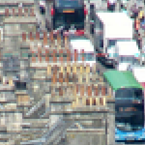
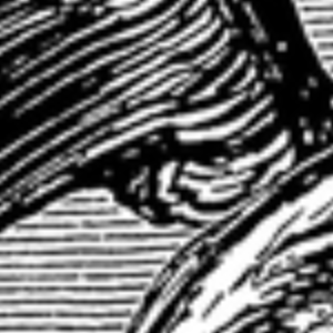
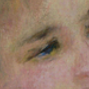
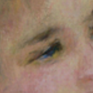
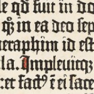
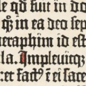
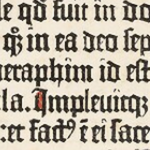
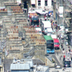
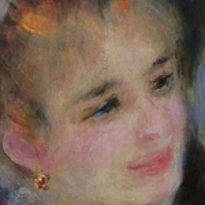
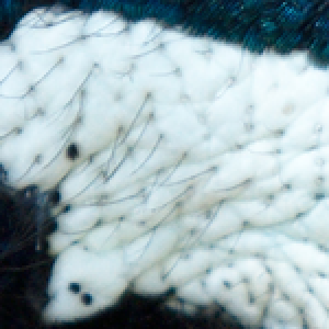
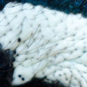
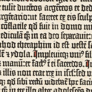
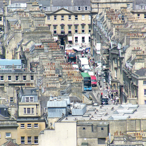
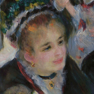
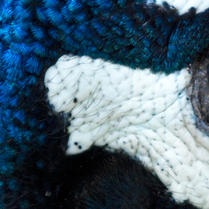
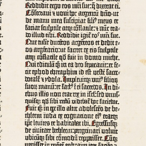
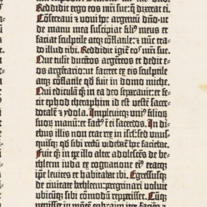
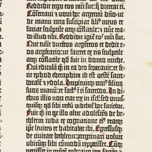
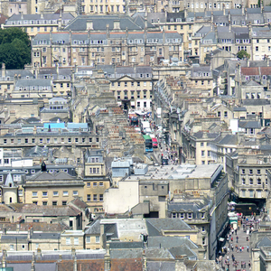
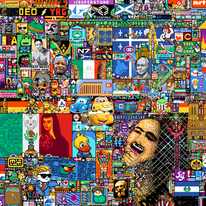
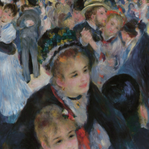
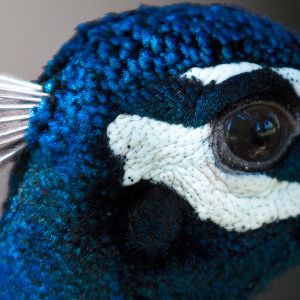
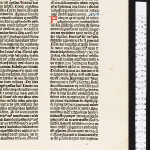
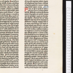
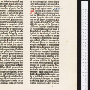
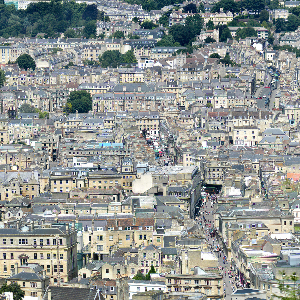
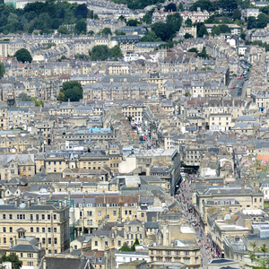
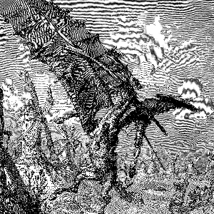
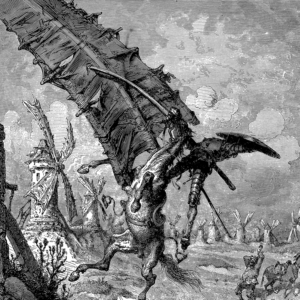
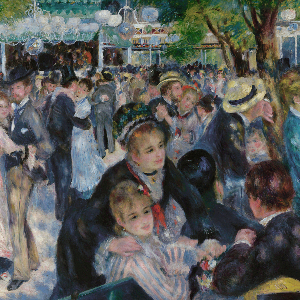
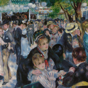
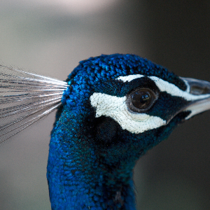
Before we begin, the images below showcase a variety of images resized with no interpolation, linear interpolation, and Lánczos interpolation. Lánczos produces non-blocky, sharp images, both when upscaling and downscaling.23
| Gutenberg | Bath | Quixote | Place | Renoir | Peacock | |||||||||||||
|---|---|---|---|---|---|---|---|---|---|---|---|---|---|---|---|---|---|---|
| Nearest | Linear | Lánczos | Nearest | Linear | Lánczos | Nearest | Linear | Lánczos | Nearest | Linear | Lánczos | Nearest | Linear | Lánczos | Nearest | Linear | Lánczos | |
| 4 |
 |
 |
 |
 |
 |
 |
 |
 |
 |
 |
 |
 |
 |
 |
 |
 |
 |
 |
| 2 |
 |
 |
 |
 |
 |
 |
 |
 |
 |
 |
 |
 |
 |
 |
 |
 |
 |
 |
| 1 |
 |
|
|
 |
|
|
 |
|
|
 |
|
|
 |
|
|
 |
|
|
| ½ |
 |
 |
 |
 |
 |
 |
 |
 |
 |
 |
 |
 |
 |
 |
 |
 |
 |
 |
| ¼ |
 |
 |
 |
 |
 |
 |
 |
 |
 |
 |
 |
 |
 |
 |
 |
 |
 |
 |
We will proceed as follows:
- A description of the problem we’re trying to solve;
- How interpolation can be phrased in terms of convolutions;
- An introduction to \mathrm{sinc}, the “best” interpolation function, together with a quick recap on Fourier transforms;
- A concrete example of interpolating with \mathrm{sinc};
- Why we can’t and shouldn’t use \mathrm{sinc} directly;
- How \mathrm{sinc} can be modified to make it work well in practice;
- Some closing thoughts.
If you’re already familiar with Fourier analysis, section 6 might still be of interest, given that it explains the main ideas behind Lánczos interpolation.
Let’s get started.
The problem #
When resizing an image, we generally have a specific target size in mind. In this post, we focus on the general problem of “filling in” the gaps between regularly spaced samples — that is, interpolating. Once we know how to interpolate between samples, we can resample at will, including downsampling and upsampling.
Let’s consider the 1-dimensional case — we’ll see shortly how to extend 1D interpolation techniques to two dimensions. Here’s a 1-dimensional signal sampled at a fixed interval:

We’ll generally call the “original” signal from which the samples are taken f(t), and refer to the input as “time” to go along with digital signal processing terminology.
Linear interpolation is just connecting the dots:

We’ll call the interpolated signal \bar{f}(t), shown above in gold. More samples mean better interpolation:

Cubic interpolation fits a third-degree polynomial between each point and generally produces a smoother, more pleasant interpolation:

If we can interpolate in one dimension, we can easily extend it to two by first interpolating along one axis, then interpolating the interpolated 1-dimensional signals:

Here, the discrete samples are colored, and the interpolated points are shown in black. Note how linear interpolation needs two samples, while cubic needs four – the number of points we need for a unique line and cubic respectively.4
We’ll only be concerned with 1-dimensional interpolation from this point forward.
Interpolation and convolution #
It is mathematically and practically helpful to frame interpolations as convolutions.
Let’s imagine that our signal f(t) is sampled at regular intervals so that they are 1/\xi apart from each other. We’ll say that \xi is the frequency at which the samples are taken – the higher the frequency, the denser the samples. We’ll also use \xi to talk about frequencies in the spectrum of f(t) later on, and relate the two.
For instance, using our previous function and \xi = 2:

We’ll refer to a single sample with f_k, where f_k is taken at time k/\xi. Given some interpolation function g, we can convolve it with our discrete samples to get an interpolated signal \bar{f}(t):
\bar{f}(t) = \sum_{k = -\infty}^{+\infty} g(t - k/\xi) \, f_k
If the sum above is a bit opaque, don’t worry, visual aid is coming shortly.
Within this framework, linear interpolation can be seen as interpolating with an appropriately scaled triangle function:

The first thing to note is that when g(t) = \mathrm{triangle}(\xi t), convolving at the sample points will not change them. Or in other words, the convolution at k/\xi will multiply f_k by 1, and all the other f_ks by 0, with the result of having \bar{f}(k/\xi) = f(k/\xi):
Let’s see this in action when \xi = 2, and t = -3/\xi:

We’re showing the interpolating function \mathrm{triangle}(t) in green, the green points are each term of the convolution sum, and the gold point is the interpolated point (that is, the sum of the green points, which is the convolution).
As you can see, the only point that contributes is f_{-3} = f(-3/2). Note that the only non-zero green point is hidden behind the gold point – since they have the same value.
Leaving the samples intact is a desirable and guiding property for interpolating functions.
Between sample points is where things get interesting:


The triangle will mix the two points to its left and right, producing the linear interpolation in the middle. Running the convolution at every point, we get back our linear interpolation:

The triangle function is a very basic option, but we’ll soon discuss a fancier interpolation function.
\mathrm{sinc}, master interpolator #
We now get talking about \mathrm{sinc}, which is the basis for Lánczos interpolation and many other interpolation filters.
\mathrm{sinc} is defined as
\mathrm{sinc}(t) = \frac{\sin t}{t}
The hole at t = 0 is plugged by setting \mathrm{sinc}(0) = 1. It looks like this:

The first good property of \mathrm{sinc} is that it interpolates well in the sense that it keeps samples intact: we have \mathrm{sinc}(0) = 1, and then we have evenly spaced zeros. By default the zeros are spaced by \pi, but we can scale it to work with any frequency \xi using \mathrm{sinc}(\pi \xi t):

Just like with \mathrm{triangle}, the samples are preserved, given the very conveniently placed zeros. But just like before, the interesting case is when we’re interpolating between samples:


I’ve centered the interpolation point to better show what happens to the sides. While \mathrm{triangle} considers only the two closest points, \mathrm{sinc} considers an infinite number of points to its left and right.
This is what the full interpolation looks like for our function:

Nice and smooth!
Beyond being a well-behaved interpolating function, \mathrm{sinc} has a second property which makes it special in this realm.
Before going forward, let’s recap on a few Fourier ingredients:
A very large class of functions can be represented as the sum of \cos \pi \xi and \sin \pi \xi oscillations (or frequencies).
The Fourier transform \mathcal{F}\{f(t)\}(\xi) of f(t) tells us “how much” of a frequency \xi is present in f(t).
\mathcal{F}\{f(t)\} uniquely determines f, and vice-versa.
\mathrm{sinc}’s Fourier transform5 looks a bit like a brick wall. Here it is compared to the spectrum of \mathrm{triangle}:6


The spectrum of \mathrm{sinc}(\pi t) is constant within 1/2, and 0 elsewhere. Or in other words, \mathrm{sinc}(\pi t) contains a constant amount of frequencies below 1/2, and no frequencies beyond that.
The spectrum of \mathrm{triangle}, on the other hand, tapers smoothly. This tapering reflects the blurring we witness when resizing images with linear interpolation.
If we increase the \xi in \mathrm{sinc}(\pi \xi t), the spectrum will widen accordingly:


With \xi = 2 the spectrum is now of width 1, although with halved magnitude. The halving is compensated by the fact that we have double the zeros (that is, double the samples when interpolating).
When we’re interpolating by convolving we’re adding up scaled versions of \mathrm{sinc}:
\bar{f}(t) = \sum_{k = -\infty}^{+\infty} \mathrm{sinc}(\xi \pi (t - k/\xi)) \, f_k
This means that the spectrum of \bar{f}(t) will also be limited to \xi/2 just like \mathrm{sinc}(\pi \xi t) is.7
Moreover, samples taken at a rate of \xi uniquely identify functions with a spectrum of width less than \xi/2. Or in other words, there’s only one function with frequencies limited to less than \xi/2 passing through a given set of samples taken at a rate of \xi.
Intuitively, what this means is that if we take enough samples, the frequencies have nowhere to hide and are fully determined by the samples.
This key fact is known as the Shannon-Nyquist sampling theorem,8 and implies that if the spectrum for f(t) is narrower than \xi/2, and if we generate \bar{f}(t) using \mathrm{sinc}(\pi \xi t), we’ll have that f(t) = \bar{f}(t).
So, if we sample densely enough, \mathrm{sinc} can reconstruct continuous signals from discrete samples perfectly! This is the sense in which \mathrm{sinc} is the “best” interpolating function, given that it is the only function with these characteristics.
We’ve gone through a lot of mathy details quickly, but what’s important to remember is:
- \mathrm{sinc} interpolates leaving samples intact;
- The spectrum for \mathrm{sinc}(\pi \xi t) is constant within \xi/2, and zero otherwise;
- Convolving adds scaled and translated versions of \mathrm{sinc}(\pi \xi t), so the spectrum of the convolution will still be constrained to \xi/2;
- The facts above, together with Shannon-Nyquist, allow \mathrm{sinc} to reconstruct signals perfectly, assuming we sample densely enough.
In the next section we’ll gain a more intuitive understanding for how this process works out.
\mathrm{sinc} in practice #
Let’s put this knowledge in action with our example function, which just so happens to be formed of three individual frequencies:
f(t) = \sin \pi \frac{t}{5} + \frac{1}{2}\cos \pi t + \frac{1}{3}\sin \pi 2 t
| \sin \pi t/5 | \frac{1}{2} \cos \pi t | \frac{1}{3} \sin \pi 2 t |

|

|

|
Usually, the Fourier transform of a function will be continuous. However, since we’re dealing with three isolated frequencies, for this signal it will not even be a proper function, but rather one impulse for each of the three frequencies. We might plot as follows:

Shannon-Nyquist tells us that that we need to sample at a frequency greater than twice the maximum frequency in the spectrum. In this case the maximum frequency is 1, so we need to sample using some \xi > 2. If we do that and convolve with a scaled \mathrm{sinc}, we should reconstruct the signal exactly:

The dramatic switch from \xi = 2 to \xi = 2.01 is no accident: our highest frequency sits right at the boundary of the spectrum, so we need to go past it to capture it.9
While I wanted to give a good intuition on why \mathrm{sinc} is such a mathematically sound interpolator, when interpolating we usually don’t really know nor care what the frequency of the original image is. However, \mathrm{sinc} is still the starting point for many interpolation functions given its ideal properties.
The problem with \mathrm{sinc} #
Now that we know about how convolving with \mathrm{sinc} interpolates points, we still face problems. The first problem is evident: to convolve with \mathrm{sinc}, we need to consider all the samples we have every time. This is clearly impractical: we’d need to look at every pixel in the input image to generate each pixel in the output!
The second problem is what happens when our spectrum is not of limited width. Let’s consider a simple stepping function, and its spectrum:

As you can see, the spectrum of \mathrm{sgn}(t) tapers but never reaches zero. This makes sense: to identify the precise moment where the function goes from -1 to +1, we’d need samples with no distance between them. So we can never reconstruct this function exactly with a finite number of samples.
That said, one might still be surprised at how poorly \mathrm{sinc} performs in situations like this:

The reconstructed signal repeatedly overshoots and undershoot our original function. These undesirable oscillations, known as Gibbs phenomenon, show up all the time in Fourier analysis when dealing with jump discontinuities and finite approximations. They are intimately related to \mathrm{sinc} – in a sense the Gibbs oscillations are all ghosts of \mathrm{sinc} in one form or another.10
Lánczos interpolation will address both problems presented in this section.
\mathrm{sinc}, chopped and screwed #
Let’s first consider the problem of \mathrm{sinc} extending into infinity, and therefore requiring to examine all samples. Our first attempt to solve this issue might be just to just set \mathrm{sinc} to zero outside a certain window:

This allows our convolution to be made up of “only” 7 terms, rather than an infinite number of terms. For images, that would be 7 \times 7 = 49 terms, given we need to go in both dimensions. Not a tiny number, but manageable.
We’ll refer to function set to zero when |t| \ge a as \langle f(t) \rangle_a:
\langle f(t) \rangle_a = \begin{cases} f(t) & \text{if}\ -a < t < a, \\ 0 & \text{otherwise}. \end{cases}
How will \langle \mathrm{sinc} \rangle_3 fare as an interpolation function? The first thing to notice is that we’re still stuck with the Gibbs oscillations in the reconstructed signal:

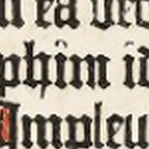
In images, this shows up in so-called “ringing” artifacts:

Those “echoes” around the letters are the same phenomenon as the wobbles in our reconstructed step function. They are particularly evident in images when text is present – the glyphs’ edges being our jump discontinuities.
However, to characterize how \langle \mathrm{sinc} \rangle_a fares mathematically we can again look at its spectrum compared to \mathrm{sinc}’s. Here’s the spectrum of \langle \mathrm{sinc} \rangle_a with a set to 3, 5, and 10 respectively:

The Gibbs oscillations spoil the fun again. Earlier, we didn’t have enough samples, this time, we have too little \mathrm{sinc}, but it’s the same phenomenon. Lánczos’ key idea was to exploit its specific nature to modify our truncated function and counteract them.11
The oscillations in the spectrum for our truncated function follow a frequency that depends directly on how wide our window is – that is, how big a is. We can immediately see this from the last plot: as we increase a, we’re getting more rapid oscillations.
We’re going to make this precise now, so we need to get a bit technical. The maths is not required to understand the intuition behind Lánczos interpolation – but it is useful to grasp the ideas that underpin it.
We’ve been throwing the Fourier transform around, but let’s define it exactly, alongside its inverse:
\begin{equation*} \begin{split} \mathcal{F}\{f(t)\}(\xi) = & \int_{-\infty}^{+\infty} f(t) \, e^{-2 \pi i \xi t} \, dt \\ f(t) = &\int_{-\infty}^{+\infty} \mathcal{F}\{f(t)\}(\xi) \, e^{+2 \pi i \xi t} \, d\xi \end{split} \end{equation*}
As usual we’re packing both \sin and \cos oscillations together using Euler’s formula:
e^{i x} = \cos x + i \sin x
The Fourier transform picks out how much a given frequency contributes to the function by looking how much they “line up”.
What we want to do is modify \langle f(t) \rangle_a so that its spectrum is as close as possible to that of f(t). Our starting point will be characterizing the nature of the error in the spectrum more precisely. First, let’s split the spectrum of f(t) in three parts:
\mathcal{F}\{f(t)\}(\xi) = \int_{-\infty}^{-a} f(t) e^{-2 \pi i \xi t} \, dt + \int_{-a}^{+a} f(t) e^{-2 \pi i \xi t} \, dt + \int_{+a}^{+\infty} f(t) e^{-2 \pi i \xi t} \, dt
The error for the spectrum of \langle f(t) \rangle_a will be the first and third term:
\mathcal{F}\{f(t)\}(\xi) - \mathcal{F}\{\langle f(t) \rangle_a\}(\xi) = \int_{-\infty}^{-a} f(t) \, e^{-2 \pi i \xi t} \, dt + \int_{+a}^{+\infty} f(t) \, e^{-2 \pi i \xi t} \, dt
These are the annoying oscillations we see for our truncated \mathrm{sinc}s, and that we do not want. Considering only the right hand side of the sum above, and reworking it a bit, we get:
\begin{equation*} \begin{split} \int_{+a}^{+\infty} f(t) \, e^{-2 \pi i \xi t} \, dt & = \int_{0}^{+\infty} f(t+a) \, e^{-2 \pi i \xi (t + a)} \, dt\\ & = e^{-2 \pi i \xi a} \int_{0}^{+\infty} f(t+a) \, e^{-2 \pi i \xi t} \, dt \end{split} \end{equation*}
We’ve now phrased the error as a modulation of the frequency e^{-2 \pi i \xi a}. Again, pause to appreciate that this “carrier wave” gets faster as a grows, which is consistent with how we witnessed our oscillations get more rapid as we truncated \mathrm{sinc} with a wider window.
Here’s the error for the spectrum of \langle \mathrm{sinc} \rangle_3, together with its carrier wave \cos 2 \pi 3 \xi:12

Lánczos’ next step was to “smooth out” the undesired oscillations by averaging out the result by the period of that frequency:
\text{smoothed} \: \mathcal{F}\{\langle f(t) \rangle_a\}(\xi) = a \int_{\xi-1/2 a}^{\xi+1/2a} \mathcal{F}\{\langle f(t) \rangle_a\}(\xi_0) \, d \xi_0
The period of e^{-2 \pi i \xi a} is 1/a, so we modify the spectrum by taking the average with a window of that width at each point.
This is what the “smoothed” spectrum looks like for \langle \mathrm{sinc} \rangle_3, \langle \mathrm{sinc} \rangle_5, and \langle \mathrm{sinc} \rangle_{10}:

It tracks the original spectrum much more closely – in fact it’s useful to focus on the area around the cutoff to see what’s going on:

The smoothed spectrum does taper a bit earlier. But this is a compromise well worth taking. Moreover, the convergence to the spectrum of \mathrm{sinc} as a grows to infinity is not compromised.
This is all well and good, but how do we apply this in practice? Well, Lánczos’ final trick was to prove that we can smooth out the spectrum of any truncated function in this way by multiplying the function pointwise with \mathrm{sinc}(\pi t / a). That’s right, it’s \mathrm{sinc} again!
So, instead of \langle f(t) \rangle_a, we’d use
\langle f(t) \rangle_a \, \mathrm{sinc}(\pi t / a)
This \mathrm{sinc} stretched to match the Gibbs oscillations is called the Lánczos window.13 Wanting to smoothen the spectrum of \langle \mathrm{sinc}(\pi t) \rangle_a itself, we’ll use
\langle \mathrm{sinc}(\pi t) \rangle_a \, \mathrm{sinc}(\pi t / a)
Lánczos interpolation consists of convolving our samples with this chopped and modified \mathrm{sinc}. This is what this new interpolation function looks like:

The plot above shows \mathrm{sinc}_3, the Lánczos window, and their pointwise multiplication. The spectrum is smoothed in exactly the way we desire. \mathrm{sinc} and its spectrum are also shown for reference.
While we set out to mimick \mathrm{sinc}’s spectrum, Lánczos interpolation actually works better than interpolating with \mathrm{sinc} in the presence of jump discontinuities, due to its dampened curve:

That said, a bit of ringing remains. This is the main drawback with Lánczos or similar filters, compared to linear interpolation or some cubic filters:
| Nearest | \langle \mathrm{sinc} \rangle_3 | \mathrm{Lanczos}_3 |
|---|---|---|
|
|
 |
|
But for many applications, Lánczos (or something close to it) will be the best compromise.
Closing thoughts #
When I set out to write this post, I wanted to work up to Lánczos interpolation using just high-school maths. I couldn’t find a way to explain it without getting quite technical, so I downgraded to an explanation targetet to an audience who has at least heard of the Fourier transform.14 That said, I still hope this post could illuminate these key areas in modern engineering through a concrete example.
Cornelius Lánczos himself brought forward a multitude of numerical methods. I highly recommend “Applied Analysis”, the book that introduced the technique explained in this post. Some of it is outdated, explaining how to manually compute roots of polynomials or solutions to linear systems. It’s still very interesting, and written in an unusual conversational style that I find endearing.
Lánczos also strikes me as a delightful man, at least from two interviews I found on YouTube about mathematics and about his life.
Another reason to write this blog post was to showcase how much one can get out of software like Mathematica when playing around with such topics. In the end I mostly used Mathematica for plots, but I encourage you to look at the notebook to get a peek of what’s possible.
Acknowledgements #
Many thanks to Alex Appetiti, Alexandru Sçvortov, Alex Sayers, Stephen Lavelle, and Kurren Nischal for reviewing drafts of this blog post.