2021-08-16 Speeding up atan2f by 50x

\mathrm{atan2} is an important but slow trigonometric function. However, if we’re working with batches of points and willing to live with tiny errors, we can produce an \mathrm{atan2} approximation which is 50 times faster than the standard version provided by glibc. Perhaps more impressively, the approximation produces a result every 2 clock cycles. This is achieved through a bit of maths, modern compiler magic, manual low-level optimizations, and some cool documents from the 50s.

The code is available in this gist, which includes details on how it is compiled.

The article will proceed as follows:

1. An overview of the problem and the results we’ll get.
2. A brief primer on what \mathrm{atan2} does, and how we will implement it.
3. Our implementation, starting from a direct C translation of the maths, followed by a series of micro-optimizations to speed it up, culminating with the fastest version.
4. Some closing thoughts.

The goal of the article is to both show how trascendental functions are computed, and how to micro-optimize guided by looking at the assembly. However, if you don’t care about how we compute \mathrm{atan2}, you can skip the second section while still understanding the optimizations process.

As usual, everything is presented without assuming much previous knowledge — in this case just basic trigonometry and C programming.

The problem #

\mathrm{atan2} is a useful trigonometric function. In short, it is needed when converting between different coordinate systems. If you don’t know what it does or how it works, worry not, we will give a primer on it later.

float atan2f(float y, float x);

void atan2_baseline(size_t num_points, const float* ys, const float* xs, float* out) {
  for (size_t i = 0; i < num_points; i++) {
    out[i] = atan2f(ys[i], xs[i]);
  }
}

This test will be our performance baseline, and our reference when it comes to evaluating the accuracy of our own versions of atan2f. Running it on one hundred thusand points gives us the following numbers:²

2.55ms,  0.33GB/s, 105.98 cycles/elem, 128.65 instrs/elem,  1.21 instrs/cycle, 27.61 branches/elem,  7.11% branch misses,  0.17% cache misses,  4.31GHz

We’re crunching the numbers at around 300MB/s, each element taking a bit more than 100 clock cycles. However it turns out that we can do a lot better than what glibc has to offer. This graph shows the performance of atan2_baseline alongside 6 other functions we will describe in the article (auto_1 to auto_4, manual_1, and manual_2):

The fastest function, manual_2, is 50 times faster than baseline, churning through more than 15GB of numbers per second, and at a throughput of less than 2 cycles per element.

This is a testament to the impact out-of-order execution, instruction-level parallelism, and vectorization. For reference, scalar floating point multiplication, a vastly simpler operation implemented in hardware, takes around 5 cycles in isolation; division takes 14-16 cycles.³

Before we start, a few caveats:

• One obvious way to improve performance when computing batches of atan2f is to split the work across threads. We won’t cover this type of optimization, focusing on single-threaded performance improvements.
• The version we’ll produce will be approximating atan2f, with a maximum error of roughly 1 / 10000 degrees, which is more than appropriate for our uses. However the techniques presented scale nicely if one needs a more precise approximation.⁴
• The code is compiled with clang++ 12.0.1. g++ 11.1.0 auto-vectorization capabilities seem to be weaker than clang++ in our case, resulting in 5-10x slower code compared to clang++ in the non manually vectorized versions.
• All the tests were ran on a Xeon W-2145, an Intel Skylake processor. The numbers are likely to be different on different microarchitectures.

Let’s get started!

Understanding and implementing \mathrm{atan2} #

If you already know what \mathrm{atan2} does and how it is defined, or don’t care about the maths, feel free to skip to the code. You won’t understand how the code works, but you will understand the optimizations in isolation.

\mathrm{atan2}: what it is and why it’s useful #

\mathrm{atan2}(y, x) gives us the angle between the ray from the origin to (x, y) and the positive x axis:

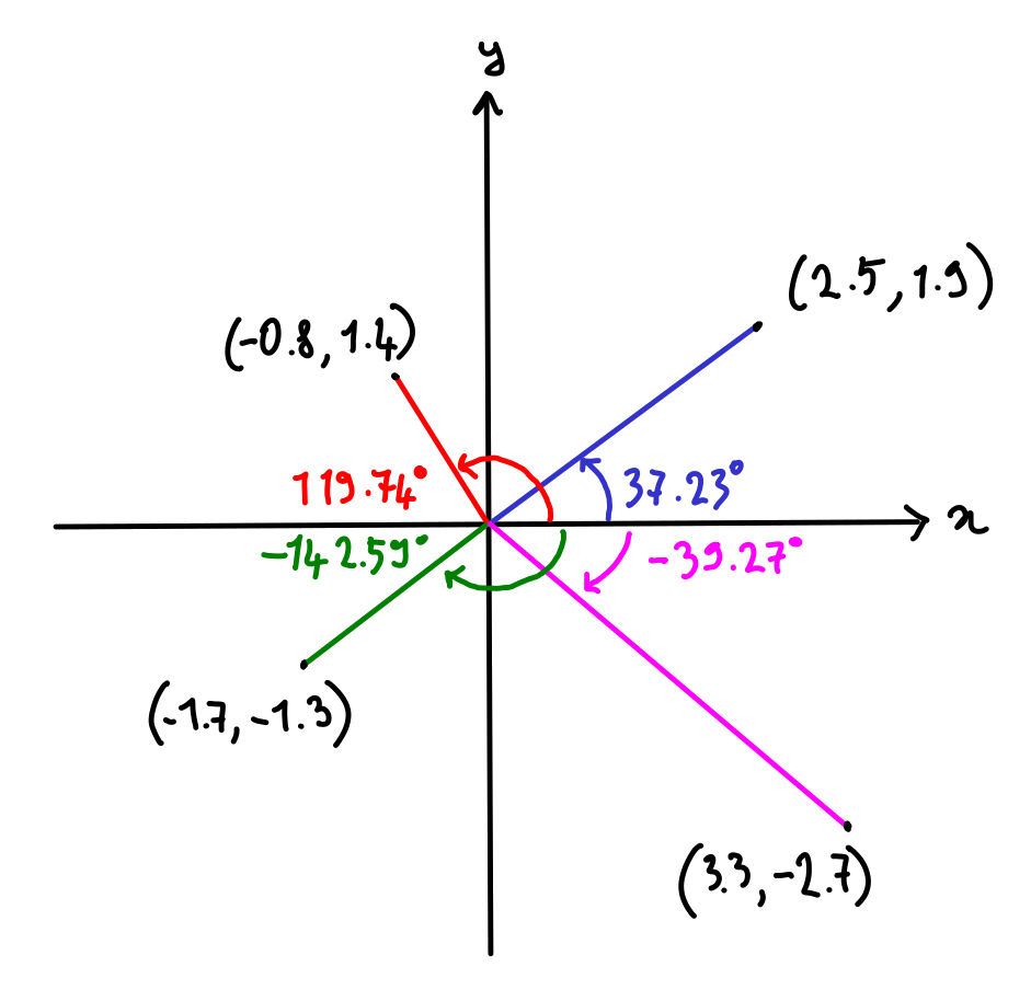
\mathrm{atan2}’s main use is to convert from cartesian coordinates to polar or spherical coordinates. In our case, \mathrm{atan2} comes up all the time when having to convert a cartesian position to its latitude and longitude.

To explain how to define it, let’s first look at a brief trigonometry recap:

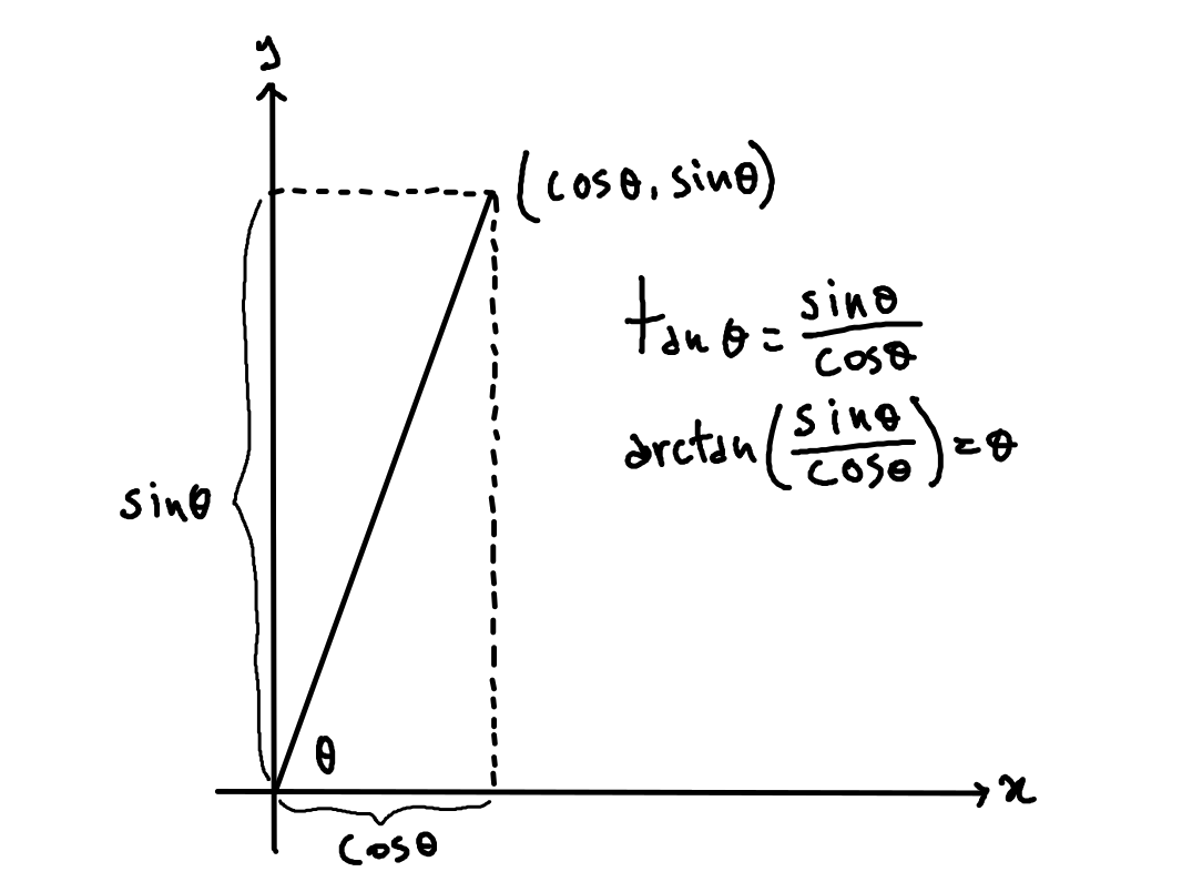
\arctan is the function we’re interested in: given the ratio between \sin \theta and \cos \theta for some angle \theta, it computes \theta.

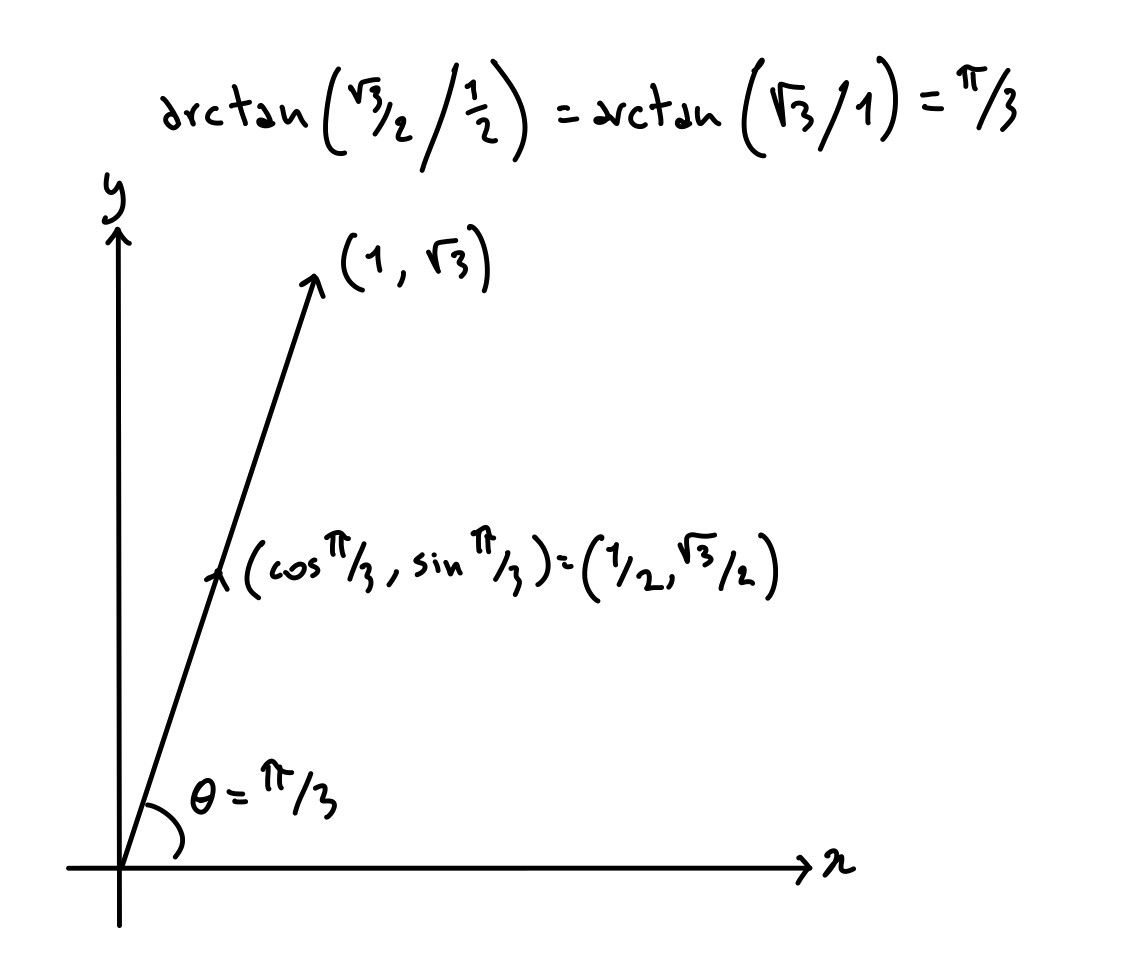
Since the argument to \arctan(\sin \theta / \cos \theta) is a ratio, \arctan(k \sin \theta / k \cos \theta) will yield the same result for any positive k. This means that \arctan(y/x) will give the angle \theta such that the ray from the origin to (\cos \theta, \sin \theta) goes through (x, y):

\mathrm{atan2}(y, x) is none other than \arctan(y / x), but with a few adjustments.

The most important adjustment is making sure to avoid the situations where the wrong result is returned after the division removes the sign information. Consider the points (1, 2) and (-1, -2). We would like \mathrm{atan2}(2, 1) to be different from \mathrm{atan2}(-2, -1), but since dividing them will yield the same result, we have a problem:

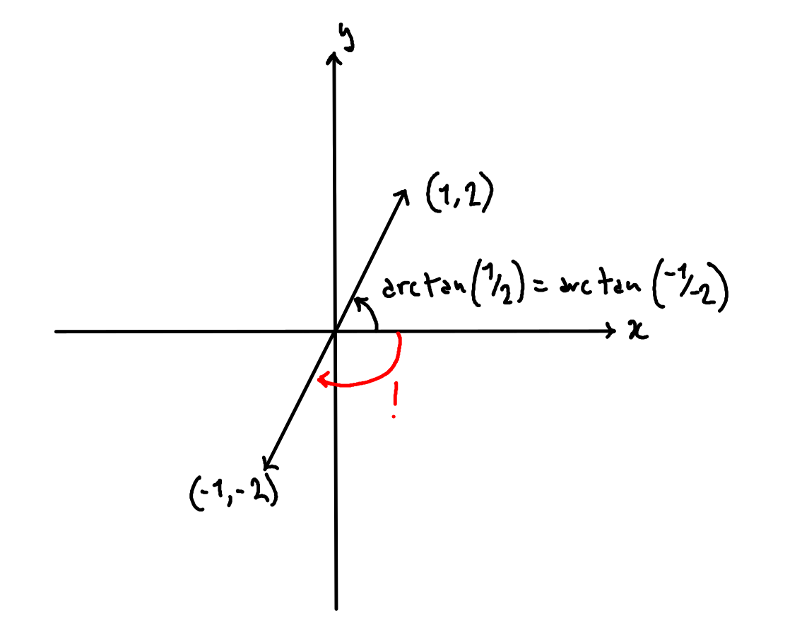
We can derive which adjustment to make to the output by analyzing what quadrant the input falls in:

The other adjustments have to do with special cases, such as when the input includes 0 or infinities. Setting those aside for the moment, we can define \mathrm{atan2}(y, x) following the diagram above:

\operatorname{atan2}(y, x) = \begin{cases} \arctan(\frac y x) & \text{if } x \ge 0 \text{ and } y \ge 0, \\ \arctan(\frac y x) + \pi & \text{if } x \lt 0 \text{ and } y \ge 0, \\ \arctan(\frac y x) - \pi & \text{if } x \lt 0 \text{ and } y \lt 0, \\ \arctan(\frac y x) & \text{if } x \ge 0 \text{ and } y \lt 0. \end{cases}

We will use this definition in our code later.

Approximating \mathrm{atan2}: why and how #

Now that we know about \mathrm{atan2}, we can explain how to compute it. x86-64 based CPUs actually have a dedicated instruction for it, part of the x87 floating-point instruction set: FPATAN. However FPATAN (and to a large extent x87 in general) has been superseded by software implementations that perform better by using newer instruction sets. In fact, the atan2f from glibc performs 50% better than the hardware FPATAN instruction.⁵

So if we eschew FPTAN and the other functions provided by the x87 instructions, we’re left with implementing \mathrm{atan2} on our own. Since we have defined \mathrm{atan2} in terms of \arctan, the first step is to figure out how to compute \arctan.

\mathrm{arctan}, like the other trigonometric functions, is a transcendental function: it cannot be expressed using only addition, multiplication, division, or square root. Unfortunately those happen to be the operations that computers can do best.

\arctan(x) = x - \dfrac{x^3}{3} + \dfrac{x^5}{5} - ... \quad (-1 \le x \le +1)

Note that the series only makes sense (converges) between -1 and +1.

If we’re looking for an approximation we can attempt to use the first few terms of the power series according to the precision that we need. Plotting the first two, three, and four terms of the power series along \arctan (in blue) gives us an idea of how much the approximations deviate from it:

Note how the more terms we keep, the better we approximate \arctan.

Nonetheless the truncated series start out good at the origin, but struggle to cover numbers close to the end points of the interval: note the gaps between the blue line and the other lines close to -1 and +1. Moreover, given that to compute \mathrm{atan2}(y, x) we need to compute \arctan(y/x) for arbitrary x and y, an approximation for [-1, +1] is not enough — we might have much bigger numbers as the argument to \arctan!

First problem: a better approximation #

While these are usually provided without source, there are several books and documents listing approximations for common functions. A particularly endearing book that serves our purpose is “Approximations for Digital Computers” by Cecil Hastings Jr., written in 1955, when “digital computers” were barely a thing.

The document explains a method to compute coefficients which minimize the maximum error of polynomial approximations, and then lists precomputed coefficients for many functions, including \arctan. Hastings lists 6 versions of increasing precision, going from 3 to 8 terms. For instance here is the least precise version, with a max error of roughly 0.03 degrees:

0.995354x -0.288679x^3 + 0.079331x^5 \quad (-1 \le x \le +1)

Note the similarity with x + -x^3/3 + x^5/5, which would be the first three terms of the power series. Plotting this approximation alongside the first three terms shows how much better it tracks \arctan:

Note how close to the endpoints -1 and +1 the approximation does not present the gap with \arctan, while the first three terms of the power series drift away sooner.

Hastings also presents a nice plot illustrating how more terms bring more precision, noting that the results are “fairly good”:

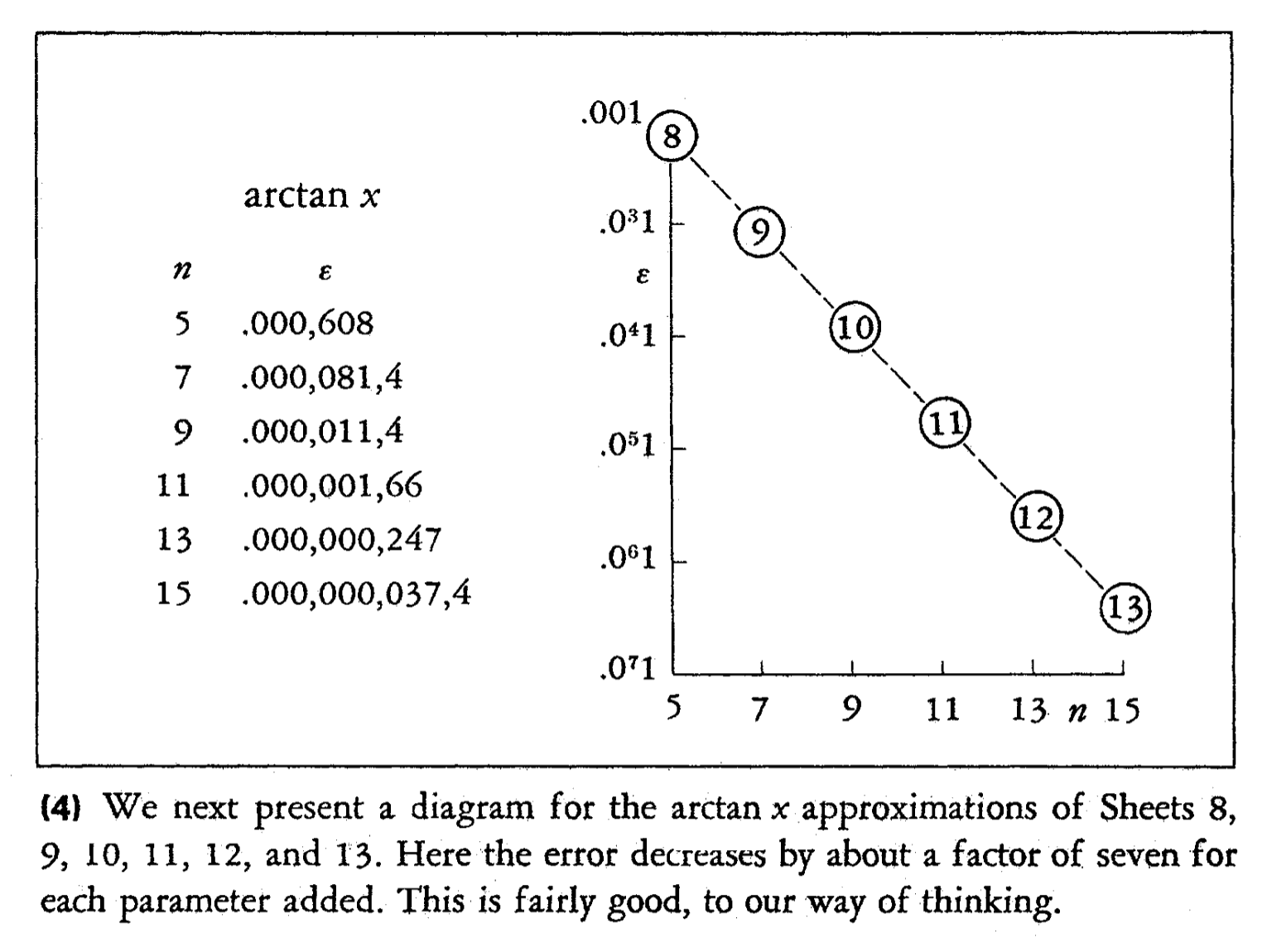
For our approximation, which we’ll call \arctan^{*}, we’ll pick the version with 6 terms, with a maximum error of roughly 1/10000 degrees:

\arctan^*(x) = a_1x + a_3x^3 + a_5x^5 + a_7x^7 + a_9x^9 + a_{11}x^{11}\\ \quad \\ \begin{array}{ll} a_1 = +0.99997726 & a_7 = -0.11643287 \\ a_3 = -0.33262347 & a_9 = +0.05265332 \\ a_5 = +0.19354346 & a_{11} = -0.01172120 \end{array}

Second problem: working between -1 and +1 #

Now that we have our \arctan approximation, we need to work around the fact that it only works if -1 \le x \le +1. We can’t easily “fix” the series to make it work beyond the current domain without making it considerably more complicated. Moreover, even if we did, we would still need an arbitrary number of terms if we wanted it to accurately work with arbitrary inputs.

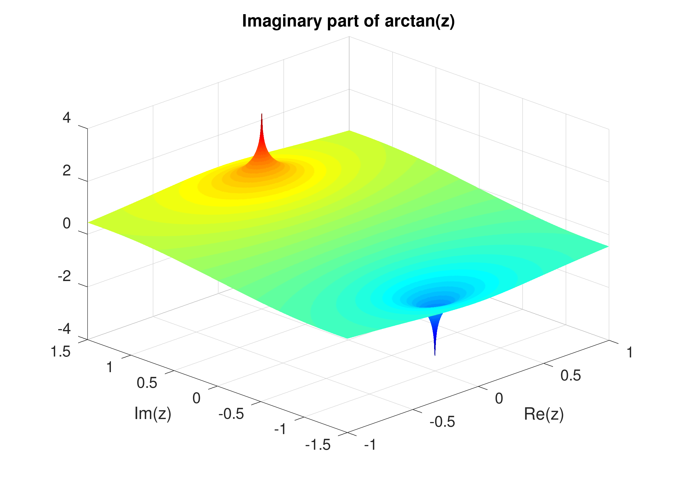
What we can do instead is avoid ever calling \arctan with inputs outside [-1, +1]. We can do that by exploiting the fact that

\begin{array}{ll} \arctan(y/x) + \arctan(x/y) = +\pi/2 & \text{if } x/y \ge 0 \\ \arctan(y/x) + \arctan(x/y) = -\pi/2 & \text{if } x/y \lt 0 \end{array}

Which can be easily verified geometrically. This allows us to compute \arctan(y/x) as follows:

\begin{array}{ll} \arctan^{*}(y/x) & \text{if } |y| \le |x|, \\ +\pi/2 - \arctan^{*}(x/y) & \text{if } |y| \gt |x| \wedge x/y \ge 0,\\ -\pi/2 - \arctan^{*}(x/y) & \text{if } |y| \gt |x| \wedge x/y \lt 0. \end{array}

By forcing the denominator to be of greater magnitude, we’ll always have an argument in [-1, +1], fitting within the domain of our approximation.

And that’s it! That is all we need to compute \mathrm{atan2}.

To recap, this is how we will proceed to compute the result of \mathrm{atan2}(y, x) in three easy steps:

1. Approximate \arctan using \arctan^{*}, using y/x or x/y as input, depending on whether |y| \le |x|;
2. If the numerator and denominator have been swapped, adjust the \arctan^{*} output as described above;
3. Adjust the output further to restore the correct quadrant and widening it from [-\pi, +\pi] to [-\pi/2, +\pi/2] as described at the beginning of this section.

Our atan2f implementations #

auto_1: A surprisingly fast first version #

inline float atan_scalar_approximation(float x) {
  float a1  =  0.99997726f;
  float a3  = -0.33262347f;
  float a5  =  0.19354346f;
  float a7  = -0.11643287f;
  float a9  =  0.05265332f;
  float a11 = -0.01172120f;

  float x_sq = x*x;
  return
    x * (a1 + x_sq * (a3 + x_sq * (a5 + x_sq * (a7 + x_sq * (a9 + x_sq * a11)))));
}

We then define the code adjusting the input and the output according to the previous section:

void atan2_auto_1(size_t num_points, const float* ys, const float* xs, float* out) {
  for (size_t i = 0; i < num_points; i++) {
    // Ensure input is in [-1, +1]
    float y = ys[i];
    float x = xs[i];
    bool swap = fabs(x) < fabs(y);
    float atan_input = (swap ? x : y) / (swap ? y : x);

    // Approximate atan
    float res = atan_approximation(atan_input);

    // If swapped, adjust atan output
    res = swap ? (atan_input >= 0.0f ? M_PI_2 : -M_PI_2) - res : res;
    // Adjust quadrants
    if      (x >= 0.0f && y >= 0.0f) {}                     // 1st quadrant
    else if (x <  0.0f && y >= 0.0f) { res =  M_PI + res; } // 2nd quadrant
    else if (x <  0.0f && y <  0.0f) { res = -M_PI + res; } // 3rd quadrant
    else if (x >= 0.0f && y <  0.0f) {}                     // 4th quadrant

    // Store result
    out[i] = res;
  }
}

We then run our benchmark:

0.21 s, 3.75GB/s, 8.29 cycles/elem, 8.38 instrs/elem, 1.01 instrs/cycle, 0.13 branches/elem, 0.01% branch misses, 0.03% cache misses, 3.89GHz, 0.000109283deg max error, max error point: -0.563291132, -0.544303775

Vectorization #

Modern CPUs include instructions to manipulate multiple values at a time. This kind of processing is usually referred to as SIMD (“single instruction, multiple data”), and code that leverages SIMD instructions is referred as vectorized.

atan2_auto_1(unsigned long, float const*, float const*, float*):
  ...                                      ; some preliminary setup
.LBB5_6:                                   ; vectorized loop starts here
  ; `rsi` = `ys`, `rdx` = `xs`, `r8` = `i`, note that the *4 is needed
  ; since a `float` is 4 bytes.
  vmovups ymm12, ymmword ptr [rsi + 4*r8]  ; load 8 elements from ys in `ymm12` AVX register
  vmovups ymm13, ymmword ptr [rdx + 4*r8]  ; load 8 elements from xs in `ymm13` AVX register
  vandps  ymm14, ymm13, ymm0               ; start computing `atan2` approximation
  ...
  add     r8, 8                            ; increase pointer offset by 8, since
  cmp     rax, r8                          ; we're processing 8 elements at a time,
  jne     .LBB5_6                          ; and resume loop if we're not done.
  ...

The instructions starting with v (like vmovups) are those operating on vectors.

So instead of loading two numbers at a time, and computing the atan2f approximation for them, it’s loading two vectors of eight numbers at a time, and computing \mathrm{atan2} for all of them in parallel. If we turn off automatic vectorization with -fno-tree-vectorize, our function will be ~6 times slower. This kind of speedup is not uncommon when taking advantage of vectorization, and we didn’t even have to know about vectorization to achieve it. Thanks, compilers!

Vectorization also explains the lack of branches. Given that the vectorized code will be working on 8 elements at a time, branches pose a challenge, since we might have to branch on some numbers of a given vector but not on others. For this reason SIMD instruction sets, including AVX, contain instructions to avoid having to explicitly branch. In fact, even just taking advantage of these instructions without processing numbers in parallel gives a considerable speedup, since it avoids expensive branch mispredictions.

One branch must remain: the one checking if the loop should continue. However, since we process 8 elements at a time, we have 1/8 = 0.125 branches per element.¹¹

While this first version is fast, we can still do much better just through micro-optimizations.

auto_2: avoid going through double #

The first improvement is an easy one, but one worth reporting to remind ourselves of two of the more annoying features of C — the preprocessor and automatic type conversion. Looking at the assembly, a series of instruction sticks out (if you’re familiar with AVX anyway):

...
vcvtps2pd       ymm14, xmm1
vextractf128    xmm3, ymm1, 1
vcvtps2pd       ymm3, xmm3
vaddpd  ymm15, ymm10, ymm3
vaddpd  ymm4, ymm14, ymm10
vcvtpd2ps       xmm4, ymm4
vcvtpd2ps       xmm5, ymm15
vinsertf128     ymm4, ymm4, xmm5, 1
...

ps is AVX-speak for float, and pd for double. What’s happening above is that we’re converting two vectors of floats to vectors of doubles (vcvtps2pd, “vector convert float to double”), performing some operations on them (vaddpd, “vector add double”), and then converting back to floats (vcvtpd2ps).

We’re not using any doubles in our code, so what is going on?

The culprits are M_PI and M_PI_2, which are defined using the C preprocessor:

# define M_PI		3.14159265358979323846	/* pi */
# define M_PI_2		1.57079632679489661923	/* pi/2 */

These literals will be of type double, since they lack the f suffix. Going back to atan2_auto_1, we have:

else if (x <  0.0f && y >= 0.0f) { res =  M_PI + res; } // 2nd quadrant
else if (x <  0.0f && y <  0.0f) { res = -M_PI + res; } // 3rd quadrant

When adding M_PI to res an automatic type conversion from the smaller float to the larger double will take place, and then a conversion back to float to update res.

This can be rectified by making sure that we never go through doubles, for example by storing M_PI and M_PI_2 as floats first:

void atan2_auto_2(size_t num_points, const float* ys, const float* xs, float* out) {
  float pi = M_PI;
  float pi_2 = M_PI_2;

  // Same as `atan_auto_1, but with `M_PI` and `M_PI_2` replaced by
  // `pi` and `pi_2`
  ...
}

And the results:

97.50ms, 8.19GB/s, 3.79 cycles/elem, 5.38 instrs/elem, 1.42 instrs/cycle, 0.13 branches/elem, 0.01% branch misses, 0.01% cache misses, 3.88GHz, 0.000109283deg max error, max error point: -0.854430377, +0.107594967

Our second version is already twice as fast as the first one.

atan_3: compare numbers once #

The next weirdness in the assembly is that we have more comparisons than we would think are needed. Focusing on the code adjusting the output, we have:

else if (x <  0.0f && y >= 0.0f) { res =  pi + res; } // 2nd quadrant
else if (x <  0.0f && y <  0.0f) { res = -pi + res; } // 3rd quadrant

We might expect the compiler to emit only one comparison involving y, since y \ge 0 is equivalent to \lnot (y \lt 0). Or is it? Let’s look at the relevant assembly:

; ymm13 = y, ymm7 = 0
...
vcmpltps        ymm14, ymm13, ymm7  ; y < 0
...
vcmpleps        ymm13, ymm7, ymm13  ; 0 <= y
...

if (x < 0.0f) {
  res = (y >= 0.0f ? pi : -pi) + res;
}

This measure will not only result in only one comparison on y, but also simplifies the compiled code further due to the easier data flow.

Integrating this smarter branching in atan_auto_3 we get:

81.48ms,  10.24GB/s,   3.04 cycles/elem,   4.13 instrs/elem,  1.36 instrs/cycle,  0.13 branches/elem,  0.02% branch misses,  0.02% cache misses,  3.89GHz,  0.000109283deg max error,  max error point: -1.000000000, +0.120253205

A further 30% increase in performance.

auto_4: fused multiply-add #

The next thing that sticks out from the assembly is how the \arctan approximation is computed. As a reminder, this is what we have in C:

x * (a1 + x_sq * (a3 + x_sq * (a5 + x_sq * (a7 + x_sq * (a9 + x_sq * a11)))));

In assembly, it looks like this:

; ymm9: result register, ymm15: x_sq, the others are the coefficients
vmulps  ymm9, ymm15, ymm1
vaddps  ymm9, ymm9, ymm2
vmulps  ymm9, ymm15, ymm9
vaddps  ymm9, ymm9, ymm3
...

x * fmaf(x_sq, fmaf(x_sq, fmaf(x_sq, fmaf(x_sq, fmaf(x_sq, c11, c9), c7), c5), c3), c1);

And the results for atan2_auto_4:

55.89ms, 14.29GB/s,  2.17 cycles/elem,  3.63 instrs/elem, 1.67 instrs/cycle, 0.13 branches/elem, 0.01% branch misses, 0.01% cache misses, 3.88GHz, 0.000109283deg max error, max error point: -0.854430377, +0.107594967

Another 35% increase in performance, and also the last one for our automatically vectorized atan2f.

Manually vectorized implementation #

Up to this point, we’ve let the compiler do all the hard work of vectorizing the code for us. This is obviously desirable since it saves us the work of coming up with the vectorized version, including annoying details such as dealing with a number of points which is not a multiple of the vector size, in which case we must process some of the dataset in a vectorized manner, and some in a scalar manner. Moreover at this point atan2f is most likely not our bottleneck anymore.

In any case, we can increase performance further by 5-10% by vectorizing the function manually. The main difference between the scalar and the vectorized version is that all the comparisons and branches are manually converted to various forms of bit twiddling and blending.

The \arctan approximation is straightforwards:

// Include intrinsics -- functions which let us acces AVX instructions.
#include <immintrin.h>

inline __m256 atan_avx_approximation(__m256 x) {
  // __m256 is the type of 8-float AVX vectors.

  // Store the coefficients -- `_mm256_set1_ps` creates a vector
  // with the same value in every element.
  __m256 a1  = _mm256_set1_ps( 0.99997726f);
  __m256 a3  = _mm256_set1_ps(-0.33262347f);
  __m256 a5  = _mm256_set1_ps( 0.19354346f);
  __m256 a7  = _mm256_set1_ps(-0.11643287f);
  __m256 a9  = _mm256_set1_ps( 0.05265332f);
  __m256 a11 = _mm256_set1_ps(-0.01172120f);

  // Compute the polynomial on an 8-vector with FMA.

  __m256 x_sq = _mm256_mul_ps(x, x);
  __m256 result;
  result =                               a11;
  result = _mm256_fmadd_ps(x_sq, result, a9);
  result = _mm256_fmadd_ps(x_sq, result, a7);
  result = _mm256_fmadd_ps(x_sq, result, a5);
  result = _mm256_fmadd_ps(x_sq, result, a3);
  result = _mm256_fmadd_ps(x_sq, result, a1);
  result = _mm256_mul_ps(x, result);

  return result;
}

And the full version, thoroughly commented to explain all the tricks:

NOINLINE
static void atan2_manual_1(size_t num_points, const float* ys, const float* xs, float* out) {
  // Check that the input plays well with AVX
  assert_avx_aligned(ys), assert_avx_aligned(xs), assert_avx_aligned(out);

  // Store pi and pi/2 as constants
  const __m256 pi = _mm256_set1_ps(M_PI);
  const __m256 pi_2 = _mm256_set1_ps(M_PI_2);

  // Create bit masks that we will need.

  // The first one is all 1s except from the sign bit:
  //
  //     01111111111111111111111111111111
  //
  // We can use it to make a float absolute by AND'ing with it.
  const __m256 abs_mask = _mm256_castsi256_ps(_mm256_set1_epi32(0x7FFFFFFF));;

  // The second is only the sign bit:
  //
  //     10000000000000000000000000000000
  //
  // we can use it to extract the sign of a number by AND'ing with it.
  const __m256 sign_mask = _mm256_castsi256_ps(_mm256_set1_epi32(0x80000000));

  // Traverse the arrays 8 points at a time.
  for (size_t i = 0; i < num_points; i += 8) {
    // Load 8 elements from `ys` and `xs` into two vectors.
    __m256 y = _mm256_load_ps(&ys[i]);
    __m256 x = _mm256_load_ps(&xs[i]);
  
    // Compare |y| > |x| using the `VCMPPS` instruction. The output of the
    // instruction is an 8-vector of floats that we can
    // use as a mask: the elements where the respective comparison is true
    // will be filled with 1s, with 0s where the comparison is false.
    //
    // Visually:
    //
    //      5 -5  5 -5  5 -5  5 -5
    //               >
    //     -5  5 -5  5 -5  5 -5  5
    //               =
    //      1s 0s 1s 0s 1s 0s 1s 0s
    //
    // Where `1s = 0xFFFFFFFF` and `0s = 0x00000000`.
    __m256 swap_mask = _mm256_cmp_ps(
      _mm256_and_ps(y, abs_mask), // |y|
      _mm256_and_ps(x, abs_mask), // |x|
      _CMP_GT_OS
    );
    // Create the atan input by "blending" `y` and `x`, according to the mask computed
    // above. The blend instruction will pick the first or second argument based on
    // the mask we passed in. In our case we need the number of larger magnitude to
    // be the denominator.
    __m256 atan_input = _mm256_div_ps(
      _mm256_blendv_ps(y, x, swap_mask), // pick the lowest between |y| and |x| for each number
      _mm256_blendv_ps(x, y, swap_mask)  // and the highest.
    );

    // Approximate atan
    __m256 result = atan_avx_approximation(atan_input);

    // If swapped, adjust atan output. We use blending again to leave
    // the output unchanged if we didn't swap anything.
    //
    // If we need to adjust it, we simply carry the sign over from the input
    // to `pi_2` by using the `sign_mask`. This avoids a more expensive comparison,
    // and also handles edge cases such as -0 better.
    result = _mm256_blendv_ps(
      result,
      _mm256_sub_ps(
        _mm256_or_ps(pi_2, _mm256_and_ps(atan_input, sign_mask)),
        result
      ),
      swap_mask
    );
    // Adjust the result depending on the input quadrant.
    //
    // We create a mask for the sign of `x` using an arithmetic right shift:
    // the mask will be all 0s if the sign if positive, and all 1s
    // if the sign is negative. This avoids a further (and slower) comparison
    // with 0.
    __m256 x_sign_mask = _mm256_castsi256_ps(_mm256_srai_epi32(_mm256_castps_si256(x), 31));
    // Then use the mask to perform the adjustment only when the sign
    // if positive, and use the sign bit of `y` to know whether to add
    // `pi` or `-pi`.
    result = _mm256_add_ps(
      _mm256_and_ps(
        _mm256_xor_ps(pi, _mm256_and_ps(sign_mask, y)),
        x_sign_mask
      ),
      result
    );

    // Store result
    _mm256_store_ps(&out[i], result);
  }
}

And the results:

52.57ms, 15.20GB/s,  2.04 cycles/elem,  3.63 instrs/elem, 1.78 instrs/cycle, 0.13 branches/elem, 0.01% branch misses, 0.03% cache misses, 3.88GHz, 0.000109283deg max error, max error point: -0.854430377, +0.107594967

Finally, the second manual function achieves a further 5% increase in performance with slightly higher instruction-level parallelism, at the cost of silently dropping inputs containing NaNs. Understanding its details is left as an exercise to the reader 🙃.

Some closing thoughts #

What have we achieved? #

Throughout the article, we’ve used sentences such as “50x faster than glibc” or “15GB/s”. It is important to stress that these numbers are pertinent to processing many elements at once. It’s similar to saying that a factory produces 1000 widgets per hour: the factory relies on an assembly line where every stage is processing widgets at the same time. This is because our CPUs work very much like an assembly line, with many things happening at once and hundreds of instructions in flight at any given time.

The speedup would look very different if we were processing 1 element, or 8 elements, or 100, rather than 100000. More concretely, a single loop iteration in our case probably spans around 100 cycles, but many loop iterations will be running at any given point in time due to out-of-order execution. Nonetheless, the performance increase is real and did make a real program much quicker.

A great tool which was recently released which can help in building a mental model of how the CPU operates is uiCA. You can paste in the assembly for any loop and uiCA will attempt to simulate how the CPU will go through it. It can also generate a simulated timeline of how instructions get executed — for example this is what it generates for the loop in atan2_manual_1.

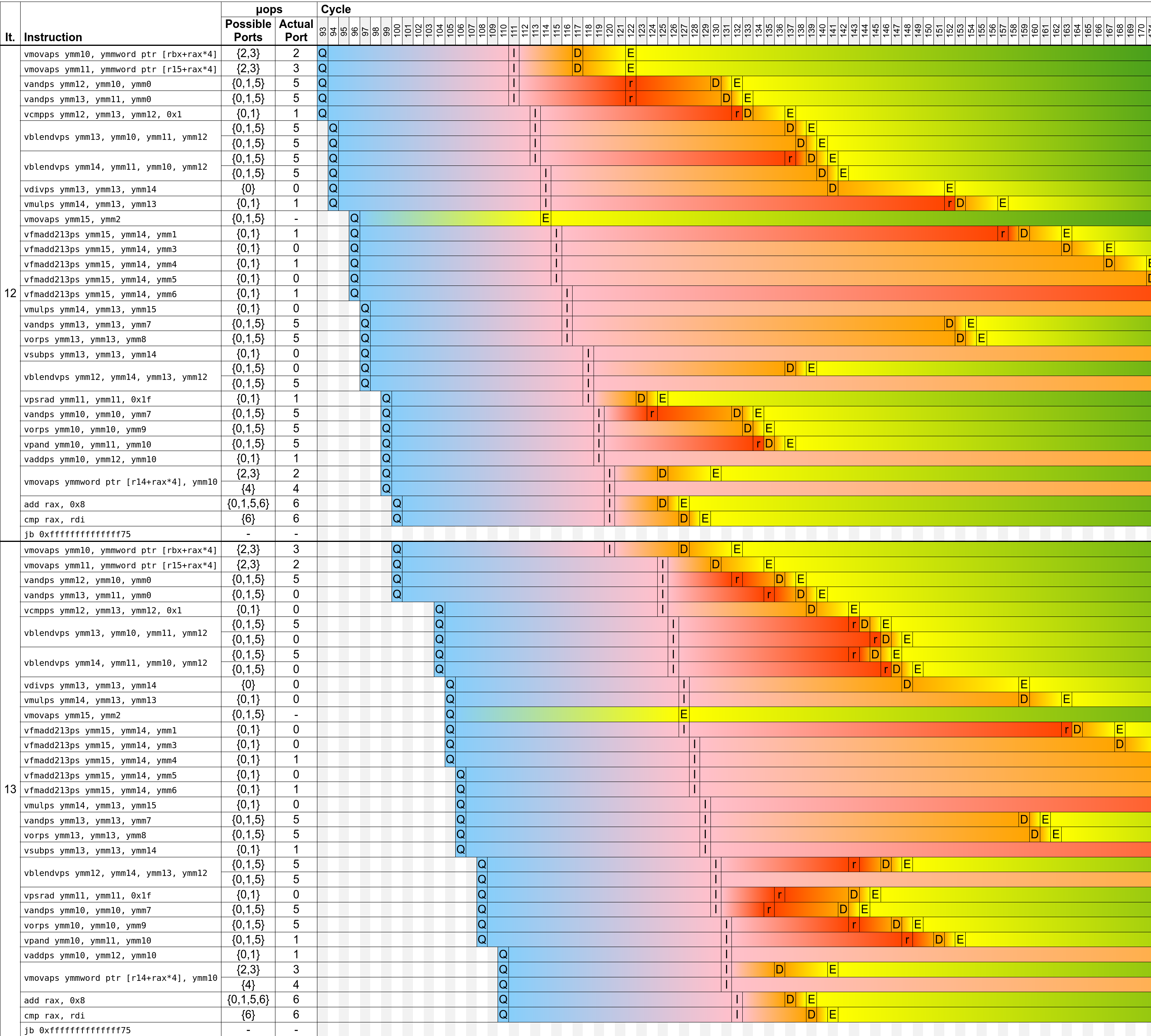
We also rely on the points being stored in row-major order — we wouldn’t be able to vectorize so effectively otherwise. In the real-world case this example is taken from, we just changed the functions generating these points (which have column-major inputs) to generate outputs in row-major.

Can we go faster? #

Maybe, although probably not much without changing the approximation. I believe the current bottleneck is fairly genuine — we’re just waiting on the CPU to crunch numbers or twiddle bits. That said it’s possible that a bit more performance could be achieved by parallelizing instructions more smartly.

Edge cases #

We’ve mostly avoided talking abouts the edge cases of \mathrm{atan2}, since they are fairly uninteresting. You can check them out on the POSIX specification for atan2.

All our functions do not handle inputs containing infinity, or when both x and y are 0, while conforming implementations must handle them specially.

As far as we can tell atan2_manual_1 handles all the other edge cases correctly. auto_1 to auto_4 do not handle inputs containing -0 in some cases, but otherwise handle all other edge cases correctly, althought they could easily be amended to do so.

atan2_manual_2 handles negative zero correctly, but silently drops NaNs unless both coordinates are NaNs. This is due to the fact that _mm256_min_ps(NaN, x) = _mm256_max_ps(NaN, x) = x. However using min and max rather than blending is what gives atan2_manual_2 the edge over atan2_manual_1. In practice, using atan2_manual_1 would be preferrable, since dropping NaNs would be extremely confusing down the line.

Acknowledgements #

Many thanks to Alex Appetiti, Stephen Lavelle, Nikola Knezevic, Karolina Alexiou, and Alexandru Scvorţov for reviewing drafts of this article and providing many helpful corrections and suggestions.